Keegan Green · kmgreen@sfu.ca

Design of an Active Knee Exoskeleton

• Read the proposal.

• Read the report.

---

Abstract

An anthropometrically-adjustable, ergonomic, active knee exoskeleton is designed — and its materials are selected — to compensate for the indirect effect of large backpack loads on hikers’ knees. This comes at the cost of weight evenly distributed over most of the leg, and that of a power source placed in the aforementioned backpack. By damping the jarring braking motion of hiking downhill, it may also regenerate energy. A motor–drivetrain pair is sized under advisement of the load’s derived speed–torque curve, and a position controller is planned to follow the knee angle curve observed over the course of the gait cycle, in a ‘moving target’ control scheme. These data were collected for design and development in a similar manner to how state feedback may be provided to the controller. Analysis is data-driven and our design is founded on research on hikers’ knee injuries, existing knee exoskeletons, and data acquisition.

---

Deriving the Speed–Torque Curve for a Knee Exoskeleton

Data analysis has been redone and improved in Python, with the help of a basis expansions module.

Data was collected for the upper and lower leg angles over the course of numerous gait cycles, walking uphill and downhill. For each case, this eventually provided me and my team with the knee angle, angular velocity, angular acceleration, the torque for a backpack load, and the speed–torque curve to to match with that of a to-be-selected motor–drivetrain pair. This would be controlled to follow a moving reference/target — the knee angle — in user-selectable incline and decline operation modes. Data analysis is documented as follows.

Requisites

• Numerical methods

• Rigid body dynamics

• Biomechanics

---

Function my_smooth()

Applies a moving average algorithm to a periodic signal, specifically for knee angular velocity and acceleration over the course of the gait cycle.

---

The first (inclusive) and last (not inclusive) extended indices for what would be a ‘circular’ array are computed:

start = - window // 2
stop  = + window // 2 + np.size(arr_p)

Note

Operation a // b is equivalent to floor(a / b) — floor/integer division.

All indices of the to-be-determined extended array arr_p and given noncircular array arr are computed:

idx   = range(start, stop)        # To be out-of-bounds *queries*, for numpy.interp().
idx_p = range(0, np.size(arr_p))  # To be within-bounds *samples*, for numpy.interp().

Function numpy.interp() supports periodic or already-repeated sample arrays. (The latter case of which might explain the need to specify a period.) This feature alone is taken advantage of, without actual interpolation:

arr = np.interp(idx, idx_p, arr_p, period = np.size(arr_p))

The moving average of the extended array is taken using a centered, constant-size window that no longer ‘overflows’ past what were the first and last indices of the original array:

return pd.Series(arr).rolling(window, center = True).mean().to_numpy()[- start : stop]

---

Function get_xy()

Derives periods \(\small T\) (seconds) of recorded gait cycles to be used in numerical differentiation, queried gait cycle fractions \(x_q\) of a cubic spline model, and their corresponding limb segment angle data \(y_q\) (degrees).

Variable Naming Convention	Meaning
Lower case	Of one or more (separated) gait cycles
Upper case, except X1 and X2	Of multiple gait cycles (not separated)
Suffix: _data	Model-ready points (input)
Suffix: q	Model query points (output)

---

A moving average algorithm is applied — mainly for convenience — to smooth out undesirable peaks of relatively ‘extreme’ value but low prominence:

Y_smooth = pd.Series(Y).rolling(window, center = True).mean().to_numpy()

\[Y_\textsf{smooth}[\,i\,]={\rm mean}\underbrace{\{\,\dots,\,Y[\,i-1\,],\,Y[\,i\,],\,Y[\,i+1\,],\,\dots\,\}}_\textsf{moving window}\]

where ... happens to just be \(\small Y[\,i\pm({\rm window}-1)\,/\,2=2\,]\) in our case (\(\small{\rm window}=5\)).

The first and last two values of Y_smooth are NaN (i.e., undefined) due to the centered, constant-size window ‘overflowing’ beyond these points instead of shrinking to fit those available. Because these values are to be discarded in our case, this is acceptable.

Note

Function pandas.DataFrame.rolling() does not properly support adjustable-width or even-valued windows, let alone non-integer ones.

An even-valued window would also be ‘split up’ between endpoint weights:

\[Y_\textsf{smooth}[\,i\,]=\frac{0.5\,Y[\,i-2\,]+Y[\,i-1\,]+Y[\,i\,]+Y[\,i+1\,]+0.5\,Y[\,i+2\,]}{4}\]

---

from scipy.signal import find_peaks

A peak finding algorithm is applied to find candidate points for splitting up individual gait cycles:

peaks, _ = find_peaks(Y_smooth)  # indices
heights = - Y_smooth[peaks]      # values (negative for convenience when sorting...)

Note

For reference: Function scipy.signal.find_peaks() also supports a minimum height, a required threshold relative to adjacent values, a minimum distance between indices, a minimum prominence, a minimum width, and a minimum plateau_size.

\(\small\rm(peaks,heights)\) is temporarily converted to a pandas ‘DataFrame’ to remove peak locations whose corresponding heights are not sufficiently ‘extreme’ for partitioning valid gait cycles:

peaks = pd.DataFrame(np.c_[peaks, heights])

          .sort_values(1)          # Sort everything by −height (ascending).
          .iloc[: cycles + 1, 0]   # Keep only relevant peak locations.
          .sort_values()           # Re-sort the filtered peak locations.

          .to_numpy().astype(int)  # Convert to a numpy array of integers for valid indexing.

DataFrame
Index	Series 0	Series 1
…	peaks — sorted 2nd	heights — sorted 1st

---

The time periods \(\small T\) (seconds) of each recorded gait cycle are also computed, where sampling frequency \(\small f_\textsf{s}=100\ \rm Hz\) (samples per second) converts from data point index to real time:

T = np.diff(peaks) / fs

Note

Function numpy.diff() does not necessarily mean numerical differentiation (e.g., in this case).

---

The following variables are initialized to empty lists such that they may be added to:

• \(\small(x,y)\) will be a pair of 2-D nested lists of gait cycle fractions and corresponding limb segment angle data for each cycle, both with redundant endpoints.

• \(\small(x_{\:\!\textsf{data}},y_{\:\!\textsf{data}})\) will be a pair of 1-D flattened lists of gait cycle fractions and corresponding limb segment angle data for all cycles, neither with redundant endpoints. These will be ready to model.

x, y, x_data, y_data = [], [], [], []

Note

The more concise x = y = x_data = y_data = [] is syntactically correct but would create shallow ‘copies’ — as opposed to true deep copies — of one empty list.

Now, for each arbitrarily positioned gait cycle, partitioned by relevant peaks:

for i in range(0, np.size(peaks) - 1):

    x.append(np.linspace(0, 1, peaks[i + 1] - peaks[i] + 1))  # Include the current gait cycle fraction.
    y.append(Y_smooth[peaks[i] : peaks[i + 1] + 1])           # Include its corresponding limb segment angle data.

    plt.plot(x[i], y[i], color = ...)                         # Add to a matplotlib plot.

    x_data = np.r_[x_data, x[i][1 :]]                         # Include the current gait cycle fraction.
    y_data = np.r_[y_data, y[i][1 :]]                         # Include its corresponding limb segment angle data.

Notes

• Function numpy.diff() can only simplify some of this.

• Method .append() is necessary for x and y, but not their _data equivalents.

• Not-technically-a-function numpy.r_[] essentially concatenates numpy.array() rows. Similarly, numpy.c_[] will concatenate columns.

The startpoints of \(\small(x_{\:\!\textsf{data}},y_{\:\!\textsf{data}})\) — initially removed for convenience — are re-included:

x_data = np.r_[x[0][0], x_data]
y_data = np.r_[y[0][0], y_data]

---

Repeat \(\small(x_{\:\!\textsf{data}},y_{\:\!\textsf{data}})\) for reps × 1 gait cycle:

X1, X2 = np.meshgrid(x1 = x_data[1 :], x2 = range(0, reps))  # X1, X2, x1, and x2 are not gait cycle fractions.

X_data = np.r_[x_data[0], np.ndarray.flatten(X1 + X2)]
Y_data = np.r_[y_data[0], np.tile(y_data[1 :], reps)]

This is explained with the aid of a simplified example:

\(x_1\)				\(x_2\)
0.1	0.2	0.3	…	0	1	2	…

\(X_1\)				\(X_2\)					\(X_1+X_2\)
Repeated by Row				Repeated by Column				Rep
0.1	0.2	0.3	…	0	0	0	…	1	0.1	0.2	0.3	…
0.1	0.2	0.3	…	1	1	1	…	2	1.1	1.2	1.3	…
0.1	0.2	0.3	…	2	2	2	…	3	2.1	2.2	2.3	…
…	…	…		…	…	…		etc	…	…	…

\({\rm flatten}(X_1+X_2)\)
1st Rep				2nd Rep				3rd Rep				etc
0.1	0.2	0.3	…	1.1	1.2	1.3	…	2.1	2.2	2.3	…	…

Note

Function numpy.meshgrid() is actually intended to generate an array of sampling points for \(\small N\)-dimensional plotting.

---

Option 1 — Function get_natural_cubic_spline_model()

from get_natural_cubic_spline_model import get_natural_cubic_spline_model

The number of knots — that is, endpoints in a cubic smoothing spline — is computed:

n_knots = 1 + knots_per_rep * reps

A natural cubic spline model is generated and ‘packaged’ in lambda function \(\small{\rm spl}(x)\):

model = get_natural_cubic_spline_model(X_data, Y_data, min(X_data), max(X_data), n_knots)

spl = lambda x: model.predict(x)

Note

Function get_natural_cubic_spline_model() contains classes AbstractSpline() and NaturalCubicSpline() from a basis expansion module by Matthew Drury.

Option 2 — Class scipy.interpolate.UnivariateSpline()

from scipy.interpolate import UnivariateSpline

Note

Class scipy.interpolate.UnivariateSpline() does not support unsorted or duplicate sample points, but it does support sample weights.

To begin using this feature, \(\small Y_{\:\!\textsf{data}}\) are pivoted with respect to \(\small X_{\:\!\textsf{data}}\), as exemplified by the following data table (observations from a fuel cell toy car experiment).

Similarly, a pivot table DataFrame (reference) is generated:

df = pd.DataFrame(np.c_[X_data, Y_data]).pivot_table(values = 1, index = 0, aggfunc = ['mean', 'count'])

DataFrame.pivot_table
Index	Series 0	Series 1
New X_data	New Y_data	Weights: w

The new \(\small X_\textsf{data}\), new \(\small Y_\textsf{data}\), and \(w\) are extracted from this new DataFrame:

X_data = df.index.to_numpy()  # (new X_data) = unique (old X_data).

Y_data = df.to_numpy()[:, 0]  # For each new X_data, (new Y_data) = mean (old Y_data).
w      = df.to_numpy()[:, 1]  # For each new X_data, weights w = … count (old Y_data).

A model is generated (already in the form of a lambda function), where \(s\) is the smoothing parameter:

spl = UnivariateSpline(X_data, Y_data, w, s = 5e4)

---

If reps % 2 != 0 (i.e., the number of repeated identical gait cycles is not even-valued):

xq = np.linspace(0, 1, nq + 1)[: -1]                         # Discard endpoint. 'Break' at x = 0.
yq = spl(xq + (reps - 1) / 2)                                # Middle cycle.

where nq is the number of query points. Otherwise:

xq1 = np.linspace(0.0, 0.5, round(nq / 2) + 1)               # Keep endpoint.
xq2 = np.linspace(0.5, 1.0, round(nq / 2) + 1)               # Keep endpoint. 'Break' at x = 0.5 only.

yq1 = spl(xq1 + reps / 2 - 0)                                # Second half of the middle-left cycle.
yq2 = spl(xq2 + reps / 2 - 1)                                # First half of the middle-right cycle.

xq  = np.r_[xq1[: -1], (xq1[-1] + xq2[0]) / 2, xq2[1 : -1]]  # One full gait cycle.
yq  = np.r_[yq1[: -1], (yq1[-1] + yq2[0]) / 2, yq2[1 : -1]]  # One full gait cycle.

xq1[0] == xq2[-1] == 0 so the latter is discarded for simplicity, but xq1[-1] != xq2[0] so the average of the two is taken for \(x_q\). The same applies to \(y_q\).

---

Plot \(\small(x_q,y_q)\) with endpoints:

line = plt.plot(np.r_[xq, 1], np.r_[yq, yq[0]], color = ...);  ...

Anterior = in front of the human subject.

---

return T, xq, yq

---

1. Downhill (_D)

Y_U_D
|
Y <――――――― limb angle data
 _U <――――― upper leg — for example
   _D <――― decline (downhill)

Variable Naming Convention	Meaning	Variable Naming Convention	Meaning
Suffix: _U	Upper leg	Suffix: _D	Decline (downhill)
Suffix: _L	Lower leg	Suffix: _I	Incline (uphill)
Suffix: _K	Knee
Suffix: _T	Trunk/Torso
Suffix: _B	Back(pack)

Variable Naming Convention	Meaning
theta → θ in Python	Angle
omega → ω	Angular velocity
alpha → α	Angular acceleration

---

1.1. Upper Leg (_U) Angle

Upper leg angle data \({\small Y}_\textsf{UD}\) (degrees), known to be representative of \(n\small=37\) gait cycles, is loaded from the GitHub repository:

Y_U_D = pd.read_csv('https://raw.github.com/keeganmjgreen/MSE-420-Project/master/data/Y_U_D.csv').to_numpy()

The corresponding gait cycle periods \({\small T}_{\:\!\textsf{UD}}\), gait cycle fractions (model input points) \(x_{q,\:\!\textsf{UD}}\), and angle data (model output points) \(y_{\:\!q,\:\!\textsf{UD}}\) are derived:

T_U_D, xq, yq_U_D = get_xy(Y_U_D, fs, window, 37, reps, knots_per_rep, nq);  ...

(At the same time, the model fit is superimposed over its plotted source data…)

---

1.2. Lower Leg (_L) Angle

Similarly, for the lower leg, with \(n\small=38\) gait cycles:

Y_L_D = pd.read_csv('https://raw.github.com/keeganmjgreen/MSE-420-Project/master/data/Y_L_D.csv').to_numpy()

T_L_D, xq, yq_L_D = get_xy(Y_L_D, fs, window, 38, reps, knots_per_rep, nq);  ...

---

1.3. Upper and Lower Leg Angles

Arbitrary gait cycle fractions are aligned/matched knowing that the leg is approximately straightened when the upper and lower leg reach minimum extension and flexion, respectively, at the same time \(t^\ast\):

\[\theta_{\:\!\textsf{U}}(t^\ast)=\min_{\stackrel{}{t}}\:\!(\theta_{\:\!\textsf{U}})\approx\min_{\stackrel{}{t}}\:\!(\theta_{\:\!\textsf{L}})=\theta_{\:\!\textsf{L}}(t^\ast)\]

θq_U_D = np.roll(yq_U_D, - np.argmin(yq_U_D))         # Perform a 'circular shift': upper leg angle data.
θq_L_D = np.roll(yq_L_D, - np.argmin(yq_L_D));  ...   # Perform a 'circular shift': lower leg angle data.

plt.plot(np.r_[xq, 1], np.r_[θq_U_D, θq_U_D[0]], ...)        # Plot with endpoints: upper leg angle data.
plt.plot(np.r_[xq, 1], np.r_[θq_L_D, θq_L_D[0]], ...);  ...  # Plot with endpoints: lower leg angle data.

---

1.4. Knee (_K) Angle

θq_K_D = θq_U_D - θq_L_D + 180;  ...

plt.plot(np.r_[xq, 1], np.r_[θq_K_D, θq_K_D[0]], color = ...);  ...  # Plot with endpoints: knee angle data.

---

θq_K_D = np.deg2rad(θq_K_D)  # Switch from degrees to radians for angular velocity and acceleration.

The mean model sampling period is computed from that of all recorded gait cycle fractions and the number of query points nq per cycle:

Ts_D = np.mean(np.r_[T_L_D, T_U_D]) / nq

The same gait cycle period is expected between the upper and lower leg, but not between uphill and downhill. This will be a step size for numerical differentiation. The gait cycle period for walking uphill (1.15 s) was consistently longer than walking downhill (1.15 s), as expected.

A 2× resolution array of gait cycle fractions is computed for supersampling 1 between even-numbered (knee angle, angular acceleration) and odd-numbered (angular velocity) centered finite difference derivatives:

x = np.linspace(0, 1, 2 * nq + 1)[: -1]

1

This is not a correct term.

---

1.5. Knee Angular Velocity

The knee angular velocity is computed using numerical differentiation, and smoothed — to reduce the noise that it introduces — where nq / fs converts from a moving average window sized for sampling to one suited for querying the model:

ωq_K_D = np.diff(np.r_[θq_K_D, θq_K_D[0]]) / Ts_D
ωq_K_D = my_smooth(ωq_K_D, window * round(nq / fs))

\(\omega_{q,\:\!\textsf{KD}}\) is ‘doubly-interpolated’, primarily for plotting near the beginning and end of the gait cycle:

ω_K_D = np.interp(x, xq + 1 / (2 * nq), ωq_K_D, period = 1);  ...

plt.plot(np.r_[x, 1], np.r_[ω_K_D, ω_K_D[0]], ...);  ...  # Plot ω_K_D with endpoints.

When \(\omega_{\:\!\textsf{KD}}\) is positive (\({\small\theta}_{\:\!\textsf{KD}}\) is increasing), the upper leg is rotating — and the torso is moving — upward. The opposite is true when \(\omega_{\:\!\textsf{KD}}<0\).

---

1.6. Knee Angular Acceleration

Similarly, for angular acceleration:

αq_K_D = np.diff(np.r_[ωq_K_D, ωq_K_D[0]]) / Ts_D
αq_K_D = my_smooth(αq_K_D, window * round(nq / fs))

α_K_D = np.interp(x, xq + 1 / (2 * nq), αq_K_D, period = 1);  ...

plt.plot(np.r_[x, 1], np.r_[α_K_D, α_K_D[0]], ...);  ...

When \(\alpha_{\:\!\textsf{KD}}\) is positive (\(\omega_{\:\!\textsf{KD}}\) is increasing), the upper leg and torso are accelerating upward. The opposite is true when \(\alpha_{\:\!\textsf{KD}}<0\).

---

1.7. Knee Drive Speed–Torque Relationship

(The subject need not be an amputee.) In this figure, the length of the topmost dashed line is assumed to be negligible. Furthermore, without knowing the shape, size, or mass distribution of a backpack and its contents, the load is approximated to be a point mass with no rotational inertia about its center.

Variable Naming Convention	Meaning
l	Length of a limb segment
d	Distance between points

Variable Naming Convention	Meaning
Greek letter ι	Rotational inertia
Greek letter τ	Torque

H   = 1.8  # Typical height of a person (meters).
m_B = 1.0  # Unity backpack load (kilograms).
g   = 9.8  # Gravitational acceleration.

l_T = (0.720 - 0.530) * H  # Length of the trunk between the hip joint and backpack point of attachment.
l_U = (0.530 - 0.285) * H  # Length of the upper leg.

The rotational inertia of backpack load \(m_B\) about the knee joint axis is computed using the parallel axis theorem and law of cosines, where \(d_{K \! B}\) is the distance between the knee and backpack point of attachment:

\[\iota_D = m_B \, d_{K \! B} ^ {\, 2} = m_B \, (l_T ^ {\, 2} + l_U ^ {\, 2} - 2 \, l_T \, l_U \cos (\theta_{U \! D} + 90 ^ \circ))\]

ι_D = m_B * (l_T ** 2 + l_U ** 2 - 2 * l_T * l_U * np.cos(np.deg2rad(θq_U_D + 90)))

Comment

Moment of inertia = mass moment of inertia = angular mass = rotational inertia. I use only the term rotational inertia because the quantity is neither a moment (torque), nor a mass — it can mean that a torque is applied (under angular acceleration), and it is merely the rotational analog of mass.

The drive torque about the knee joint axis is computed for the required acceleration:

\[\tau_{K\!D} = \iota_D \, \alpha_{K \! D} + m_B \, l_U \cos(\theta_{U \! D}) \, g\]

τq_K_D = ι_D * αq_K_D + m_B * l_U * np.cos(np.deg2rad(θq_U_D)) * g

A plot of \(\small |\tau_{K \! D}|\) against \(\small |\omega_{K \! D}|\) — namely, the speed–torque curve required for the knee drive — is generated:

plt.plot(abs(τq_K_D), abs(ωq_K_D), ...)

Each point \(\small (|\tau_{K \! D}|, |\omega_{K \! D}|)\) along the speed–torque curve is written to a CSV file, initially for use with MATLAB’s interactive plotting features:

writer = csv.writer(open('_D.csv', 'w', newline = ''))

writer.writerows([['abs(τq_K_D)', 'abs(ωq_K_D)']])          # headers
writer.writerows(np.c_[abs(τq_K_D), abs(ωq_K_D)].tolist())  # columns

Now using MATLAB (Appendix), the speed–torque curve ‘envelope’ is generated:

Knee Drive Speed–Torque Curve

4.7738 rad/s² and 56.0857 N-m are the minimum required no-load speed and stall torque of the knee drive, respectively.

Knee Drive Power Curves

---

2. Uphill (_I)

---

2.1. Upper Leg (_U) Angle

Upper leg angle data \({\small Y}_\textsf{UI}\) (degrees), known to be representative of \(n\small=34\) gait cycles, is loaded from the GitHub repository:

Y_U_I = pd.read_csv('https://raw.github.com/keeganmjgreen/MSE-420-Project/master/data/Y_U_I.csv').to_numpy()

The corresponding gait cycle periods \({\small T}_{\:\!\textsf{UI}}\), gait cycle fractions (model input points) \(x_{q,\:\!\textsf{UI}}\), and angle data (model output points) \(y_{\:\!q,\:\!\textsf{UD}}\) are derived:

T_U_I, xq, yq_U_I = get_xy(Y_U_I, fs, window, 34, reps, knots_per_rep, nq);  ...

(At the same time, the model fit is superimposed over its plotted source data…)

---

2.2. Lower Leg (_L) Angle

Similarly, for the lower leg, with \(n\small=38\) gait cycles:

Y_L_I = pd.read_csv('https://raw.github.com/keeganmjgreen/MSE-420-Project/master/data/Y_L_I.csv').to_numpy()

T_L_I, xq, yq_L_I = get_xy(Y_L_I, fs, window, 38, reps, knots_per_rep, nq);  ...

---

…and so on and so forth as in Section 1.

---

Appendix

MATLAB

close

[x, y] = readvars('_D');

[x_max, i_x_max] = max(x);
[y_max, i_y_max] = max(y);

x_min = x(i_y_max);
y_min = y(i_x_max);

f = @(x, y) ((x - x_min) ./ (x_max - x_min)) .^ 2 + ((y - y_min) ./ (y_max - y_min)) .^ 2 - 1;

figure('Color', 'w', 'MenuBar', 'none')

box on
grid on
hold on

plot([     0, x_min ], [ y_max, y_max ], 'Color', '#087F23', 'LineWidth', 1)
plot([ x_max, x_max ], [ y_min,     0 ], 'color', '#087F23', 'LineWidth', 1)

fimplicit(f, [x_min, x_max, y_min, y_max], 'color', '#087F23', 'LineWidth', 1)

xlim([ 0, 100 ])
ylim([ 0,   5 ])

xticks([ 0, x_max ])
yticks([ 0, y_max ])

xlabel({'', 'Torque (N-m)', ''})
ylabel({'', 'Speed (rad/s²)'})

title({'', 'Downhill — Knee Drive', ''})

set(gca, 'FontName', 'Consolas')

print('ω_vs_τ_K_D′', '-dsvg')

MATLAB

clearvars

[x, y] = readvars('_D');

[x_max, i_x_max] = max(x);
[y_max, i_y_max] = max(y);

x_new = [x_max; x(i_x_max : i_y_max); 0];
y_new = [0; y(i_x_max : i_y_max); y_max];

figure('Color', 'w', 'MenuBar', 'none')

% Plot speed vs torque:

    subplot(2, 2, 3)

    plot(x_new, y_new, 'Color', '#087F23', 'LineWidth', 1)

    box off
    grid on
    axis equal square

    xlim([0, x_max])
    ylim([0, y_max])

    xticks(xlim)
    yticks(ylim)

    yticklabels([min(ylim), "  " + max(ylim)])

    xlabel({'', 'Torque (N-m)', ''})
    ylabel('Speed (rad/s²)')

    set(gca, 'FontName', 'Consolas')

% Plot speed vs power:

    subplot(2, 2, 4)

    plot(x_new .* y_new, y_new, 'Color', '#087F23', 'LineWidth', 1)

    box off
    grid on
    axis equal square

    ylim([0, y_max])

    xticks(xlim)
    yticks(ylim)

    yticklabels('')

    xlabel({'', 'Power (W)', ''})

    set(gca, 'FontName', 'Consolas')

% Plot power vs torque:

    subplot(2, 2, 1)

    plot(x_new, x_new .* y_new, 'Color', '#087F23', 'LineWidth', 1)

    box off
    grid on
    axis equal square

    xlim([0, x_max])

    xticks(xlim)
    yticks(ylim)

    xticklabels('')

    ylabel('Power (W)')

    set(gca, 'FontName', 'Consolas')

print('ω_vs_τ_K_D″', '-dsvg')

---

---

Knee Angle Data Logger

I mentioned in my team’s report that we considered using a quadrature encoder built into a servo motor for recording both speed and direction of the knee, but I decided against it because of its gearbox’s mechanical resistance to what would otherwise be ‘natural movement’. Months after the main project, I decided to design and construct a piece of wearable tech — an optionally-wireless knee angle data logger — to verify or disprove this assumption, for starters.

Wearing the knee angle data logger:

Wearing and testing the knee angle data logger by walking around and quickly flexing the knee at different angles:

---

It turns out that this likely has less of an effect than initially thought. In contrast, however, the lack of mechanical compliance even with at least some material flexibility, and the heavy rotational inertia of the device about the leg as it sways, are issues. In future work, the latter may be largely solved by making the sizable prototype of its data acquisition electronics more compact and/or offloading it elsewhere along and closer to the leg.

---

The device consists of the following.

• An ergonomic fabric cuff/brace that velcro-straps around the leg — above, below, and at the knee.

• An almost-servo motor (with a built-in quadrature encoder) — its housing and axle spanning the brace.

• A microcontroller ‘unit’ (MCU) — in part to convert the encoder signals to an updated value of the knee angle.

• A wireless transceiver — to transmit knee angle data to a phone.

• Two rechargeable LiPo batteries — to power the MCU and the transceiver via the MCU.

• A mini protoboard — to connect the previous three electrical parts/components.

❶ Generic representation of the servo motor (with a built-in but externally accessible quadrature encoder) — its housing and axle (❷) spanning the knee brace.

❸ The servo motor’s ‘six-position’ (6P) proprietary connection — or rather, a generic six-pin–header representation thereof.

❹ The pinout of ❸ and ❺ is as follows.

	Motor Negative		to MCU GND — Encoder Ground		Encoder Channel A
	Motor Positive		to MCU 5V0 — Encoder Power*		Encoder Channel B

❺ The servo motor’s ‘six-conductor’ (6C) proprietary cable — a narrow ribbon cable.

❻ An Arduino MCU.

❼ MCU header pins — Digital I/O: (14 total)

• RX<0 receives via UART from a computer connected via USB OR from the Bluetooth module to the MCU, one communicating device at a time.

• TX>1 transmits via UART from the MCU to a computer connected via USB AND to the Bluetooth module, at the same time.

• 2 receives the Encoder Channel B signal.

• 4 receives the Encoder Channel A signal.

• 5 is the enable input for transmitting knee angle data versus pausing the ‘transmission loop’.

❽ MCU header pins — Power:

• Vin is the 7–12-V input to the MCU, thereby also to the servo motor’s encoder and the Bluetooth module.

• GND is the voltage ground.

• 5V0 is the 5.0-V (operating voltage) supply from the MCU.

• RESET temporarily ceases running any onboard program upon being shorted to ground.

❾ Power input port (2.1-mm center-positive connector) — not in use.

❿ USB (standard B) port — optional use with cable (⓫).

⓬ Mini protoboard (no bus strips, 17 rows of terminal strips, 170 tie points).

⓭ Set-length solid-core insulated protoboard wire (⓮ two are uninsulated).

⓯ (Brown) two resistors (1, 2 kΩ).

⓰ DPDT and ⓱ SPST dual in-line package (DIP) switches (see Appendix).

⓲ Two four-pin headers (actually laid flat against the protoboard) for the Bluetooth module and batteries.

⓳ Two pairs of battery leads.

⓴ Bluetooth module.

---

System Level Block Diagrams and Technical Details

---

Programming the Microcontroller

• The computer transmits information (a program from the Arduino IDE, in the above case) to the Arduino microcontroller (and vice-versa, albeit little in the above case) via USB.

• “USB-to-UART” is actually part of an IC onboard the microcontroller.

• USB 2 here uses half-duplex (two-way) serial communication and differential signaling.

• UART uses full-duplex (simultaneous two-way) serial communication.

• UART = Universal Asynchronous Receiver-Transmitter communication protocol.

---

Programming the BLE Module

• The computer transmits information (BLE module configuration AT commands from any serial monitor, in the above case) to the BLE module (and vice-versa) through the microcontroller via USB.

• Again, “USB-to-UART” and “UART-to-USB” are actually parts of an IC onboard the microcontroller. This IC is ‘tied’ to the microcontroller TX and RX pins.

• TX transmits via UART from the labeled device.

• RX receives via UART from a communicating device.

• *using a voltage divider with a 1-kΩ resistor from 5.0 V to 3.3 V and a 2-kΩ resistor from 3.3 V to ground (microcontroller GND pins).

The logical high voltage levels of the microcontroller and BLE module are around 5.0 V (microcontroller 5V0 pin) and 3.3 V (microcontroller 3V3 pin), respectively.

As such and in this one case, not using a level shifter such as an equivalent voltage divider or transistor equivalent may damage the BLE module.

• BLE = Bluetooth Low Energy.

---

Logging Knee Angle Data (Default Operation Mode)

• Technically-not-a-servomotor (No built-in feedback control of position or speed.)

• Actuator: DC motor with gear train.

• Sensor: Optical Rotary Encoder (reference) in quadrature.

• For position feedback or just sensing (in this case).

• Encodes direction as well as knee angle increments/decrements (0.5° resolution).

• Transparent disc with two opaque, circular ‘barcodes’ offset from each other by 0.5°.

• LED–photodiode pairs placed across these patterned ‘light-slots’.

• Outputs two digital signals.

• Arduino Duemilanove Microcontroller.

• Receives encoder signals on digital pins “A” and “B”.

• Decodes knee angle from encoder output.

• UART-to-BLE = DSD TECH HM-10 Master and Slave Bluetooth 4.0 LE Module.

• Connected to the microcontroller TX and RX pins.

• Android Phone.

• Serial Bluetooth Terminal, by Kai Morich.

• Windows 10 Computer.

• Knee Angle Data Logger Interface, by me.

---

Appendix

Switch Position 1	Functionality	Functionality
Switch 6 · ON	Shorts MCU RESET to MCU GND	Resets the MCU (temporarily)
Switch 5 · ON	Shorts 7.4 V to MCU Vin	Powers on the device
Switch 4 · ON	Shorts BLE module GND to MCU GND	Powers on the BLE module thereafter
Switch 3 · OFF	Breaks MCU GND to digital pin 5	Enables knee angle data transmission (default operation mode)
Switch 2 · ON	Shorts the MCU TX to BLE module RX by default	Enables wirelessly transmitting data — logging knee angle data
Switch 1 · ON	Shorts the MCU RX to BLE module TX by default	Enables wirelessly receiving data
Switch 0 · C2	Sets the MCU TX/RX to connect to BLE module RX/TX	Enables logging knee angle data (default operation mode)
Switch 0 · C1	Sets the MCU TX/RX to connect to BLE module TX/RX	Enables programming the BLE module

1

Switch 0 is DPDT (double-pole, double-throw). Switches 1–6 are SPST (single-pole, single-throw). (Switches 7–8 are kept closed, 7 as a jumper.)

---

kneeAngleDataLogger.ino

#include <arduino-timer.h>

int pinA = 4; // Pin for Encoder Channel A.
int pinB = 2; // Pin for Encoder Channel B.

bool oldA; // Old Encoder Channel A signal.
bool oldB; // Old Encoder Channel B signal.

bool newA; // New Encoder Channel A signal.
bool newB; // New Encoder Channel B signal.

float numDegrees = 0; // Current knee angle (relative — incremental encoder) (0.5° resolution).

// strDegrees = "±XXX.X\n"
char strDegrees[7]; // charsPerMessage = 7

int bitsPerSecond = 9600; // Default baud (data transfer) rate.
// Reliable over Bluetooth.

\(\small \; \vdots\)

\(\small \: \bullet \quad \quad \text{bits per second} = 9\,600\)

\(\small \: \bullet \quad \quad \text{start bits per character} = 1\)

\(\small \: \bullet \quad \quad \; \! \text{data bits per character} = 8\)

\(\small \: \bullet \quad \quad \: \text{stop bits per character} = 1\)

\(\small \: \bullet \quad \quad \text{bits per character} = ( \text{start bits} + \text{data bits} + \text{stop bits} ) \ \text{per character} = 10\)

\(\small \: \bullet \quad \quad \text{seconds per character ($\,T_\textsf{character}$)} = \text{bits per character} \: / \: \text{bits per second} \approx 0.001\,04\)

\(\small \: \bullet \quad \quad \text{characters per message} = 7\)

\(\small \: \bullet \quad \quad \text{seconds per message ($\,T_\textsf{message}$)} = \text{seconds per character} \, \cdot \: \text{characters per message} \approx 0.007\,3\)

\(\small \: \bullet \quad \quad \text{milliseconds per message} = \lceil \, \text{seconds per message} \: \cdot \, 10^3 \, \rceil = \lceil \, 7.3 \, \rceil = 8 \longrightarrow \boxed{10}\)

\(\small \; \vdots\)

/*
 * int startBitsPerChar = 1;
 * int  dataBitsPerChar = 8;
 * int  stopBitsPerChar = 1;
 *
 * int bitsPerChar = startBitsPerChar + dataBitsPerChar + stopBitsPerChar;
 *
 * float secondsPerChar = bitsPerChar / bitsPerSecond;
 *
 * int charsPerMessage = 7;
 *
 * float secondsPerMessage = secondsPerChar * charsPerMessage;
 *
 * int millisPerMessage = ceil(secondsPerMessage * 1e3);
 *
 */

int millisPerMessage = 10;

Timer<1, millis, char *> timer;

void setup()
{
    pinMode(pinA, INPUT_PULLUP);
    pinMode(pinB, INPUT_PULLUP);
    pinMode(5,    INPUT_PULLUP);

    oldA = digitalRead(pinA);
    oldB = digitalRead(pinB);

    Serial.begin(bitsPerSecond);

    timer.every(millisPerMessage, [](char *strDegrees) -> bool { Serial.println(strDegrees); return true; }, strDegrees);
}
void loop()
{
    if (digitalRead(5))
    {
        timer.tick();
    }

    dtostrf(numDegrees, 3, 1, strDegrees);

    newA = digitalRead(pinA);
    newB = digitalRead(pinB);

    if ((!oldA && newB || oldA && !newB) &&
    (!oldB && !newA || oldB && newA))
    {
        numDegrees += 0.5;
    }
    if ((oldA && newB || !oldA && !newB) &&
    (!oldB && newA || oldB && !newA))
    {
        numDegrees -= 0.5;
    }
    oldA = newA;
    oldB = newB;
}

---

kneeAngleDataLoggerInterface.ipynb

Knee Angle Data Logger Interface

I developed a Windows 10 interface in Python for the knee angle data logger with a wired connection to a computer. The program may be run directly by launching kneeAngleDataLoggerInterface.pyw or, naturally, by executing the following command.

$ python kneeAngleDataLoggerInterface.pyw

The interface prompts you to connect the knee angle data logger (via USB) if it has not already been connected, notifies that the device was connected, reads from the device over serial communication, and finally notifies that the device was disconnected (all Subsection 2). It then prepares the collected knee angle data (Subsection 3). Lastly, it makes the results accessible through a beautiful, interactive, in-browser plot (Subsection 4).

These features can be broken down by going through its library imports as follows.

1. Library Imports in Order of Appearance

The user is to at least be notified that the knee angle data logger was connected and disconnected (via USB). win10toast by Jithu Jacob is a Python library (PyPI, GitHub) for displaying Windows 10 toast notifications.

xxxxxxxxxx
from win10toast import ToastNotifier

On the other hand, plyer.notification shows new notification senders for every notification sent.

For reasons that will become apparent, timer functionality is to be used. time is a standard Python library (Python documentation) for time access (and conversions, for that matter).

xxxxxxxxxx
from time import time

To read from the knee angle data logger, serial communication is to be used. pySerial by Chris Liechti is a Python library (PyPI, GitHub, documentation) that encapsulates access to computer serial ports, including emulated ones such as those created by USB.

xxxxxxxxxx
from serial import Serial

The received knee angle data is to be prepared before being made accessible.

xxxxxxxxxx
import numpy  as np
import pandas as pd

pandas, for instance, can be used to calculate a moving average to smooth the knee angle data.

The prepared knee angle data is to be made accessible through a beautiful, interactive, in-browser plot. plotly by the technical computing company of the same name is a Python library (PyPI, documentation) used to style interactive graphs.

xxxxxxxxxx
import plotly.graph_objects as go

2. Minimal User Interface | Reading from the Knee Angle Data Logger

To start with, initialize an instance of the toast notifier class using a memorable name:

xxxxxxxxxx
toaster = ToastNotifier()

This class has a show_toast method which is to be used. Among other arguments, it accepts a notification title, a notification msg, and an optional boolean specifying whether or not the showing of the notification (in its entire duration) is to be threaded (reference) with further Python instructions in this module (which calls show_toast). I found that the notification message itself (not its title) is actually optional, being truly omitted by specifying msg to be a non-empty ‘empty’ string such as ' '. Method show_toast returns a boolean representing whether a notification is sent successfully or not (i.e., if one is already being shown, at least from Python). I also found that initializing multiple instances of the ToastNotifier class does not allow multiple corresponding notifications to appear simultaneously in the same way.

Now, specify the chosen 9600 / 8-N-1 serial communication (COM) port:

xxxxxxxxxx
port = 'COM4'

Try to open this serial port with the assumption that the knee angle data logger has been connected to the computer via USB:

xxxxxxxxxx
try:
│   ser = Serial(port)

If Serial cannot open the specified port (i.e., if the above assumption was incorrect), it raises a SerialException error, which is caught (handled) by the following to-be-completed block of code.

xxxxxxxxxx
except:

Now, I assume the general case that a system notification may already be present.
As such, keep trying to…

• show the user a prompt to connect to the knee angle data logger, or
• open the serial port assuming that the device has since been connected,

whichever happens first (that is, whichever the program encounters first):

xxxxxxxxxx
│   while True:
│   │
│   │   if toaster.show_toast('Connect to the knee angle data logger via USB', ' ', 
│   │   │                     threaded = True):
│   │   │   break
│   │
│   │   try:
│   │   │   ser = Serial(port)
│   │   │   break¹
│   │   except:
│   │   │   pass

¹ This break will not be reached unless the previous line, ser = Serial(port), succeeds.
At least in this context, break and pass specifically mean ‘stop trying’ and ‘skip error handling’, respectively.

↑ The first possible notification.

The device may have been connected by this point, in which case the connection prompt would be withheld.
Now, check if the ser object is defined (i.e., if the serial port was opened):

xxxxxxxxxx
│   try:
│   │   ser

If not, keep trying to open the port assuming that the device will be connected:

xxxxxxxxxx
│   except:
│   │
│   │   while True:
│   │   │
│   │   │   try:
│   │   │   │   ser = Serial(port)
│   │   │   │   break
│   │   │   except:
│   │   │   │   pass

The knee angle data logger has been connected by this point, with or without a prompt to the user.

A notification that the device was connected is to be sent. I assume that an arbitrary notification may already be present, including but by no means limited to the connection prompt from before. If this is the case, it would delay the notification that the device was connected until ‘timing out’ (for lack of a better term). With this kind of notification, the user should know the time since its corresponding event actually occurred.

As such, start a ‘timer’ (i.e., log the current time connected_tick):

xxxxxxxxxx
connected_tick = time()

Subsequently,

• keep updating the suspected end time connected_tock and the elapsed time calculated from it,
• keep trying to show a notification that the knee angle data logger was connected and of how long ago this event actually occurred,
  and
• keep checking if the serial port can be read from (i.e., if the device was not since disconnected),

all until the notification is sent:

xxxxxxxxxx
while True:
│
│   connected_tock = time()
│   connected_time = connected_tock - connected_tick
│
│   if toaster.show_toast('Knee angle data logger connected %.1f seconds ago'
│   │                     % connected_time,
│   │                     'Starting now, you may disconnect',
│   │                     threaded = True):
│   │   break
│
│   try:
│   │   ser.readline()
│   except:
│   │   try:
│   │       disconnected_tick
│   │   except:
│   │       disconnected_tick = time()

↑ The second possible notification.

The user would be ‘permitted’ to disconnect the device as soon as it is connected if the previous busy waiting while loop is manually (albeit awkwardly) threaded with the upcoming data logging one, or if done using the threading standard Python module (documentation) instead. However, the user should know not when the device is simply plugged in (as they do and need not be notified), but when the serial communication link is established soon thereafter.

Now, initialize an empty list of lines to be read from the serial port, assuming that it is still open:

xxxxxxxxxx
lines = []

Keep trying to read ASCII characters from the serial port, and add them to the list of lines thereof, until the port is no longer open (i.e., until the device is disconnected):

xxxxxxxxxx
while True:
│
│   try:
│   │   lines.append(ser.readline())
│   except:
│   │   break

Now, check if a variable disconnected_tick is already defined (i.e., if the device was disconnected while waiting to send the previous notification):

xxxxxxxxxx
try:
│   disconnected_tick

If not, start another ‘timer’ (i.e., log the current time disconnected_tick):

xxxxxxxxxx
except:
│   disconnected_tick = time()

Keep trying to show a notification that the knee angle data logger was disconnected, and of how long ago this event actually occurred:

xxxxxxxxxx
while True:
│
│   disconnected_tock = time()
│   disconnected_time = disconnected_tock - disconnected_tick
│
│   if toaster.show_toast('Knee angle data logger disconnected %.1f seconds ago' % disconnected_time, ' ', threaded = True):
│   │   break

↑ The third possible notification.

3. Preparing the Collected Knee Angle Data

See the following numbered, broken-down block of code.

Now,

1. Trim the last two line-ending ASCII characters: line feed <LF> b'\n' and carriage return <CR> b'\r'.

2. Typecast (convert) the remaining ASCII characters from a byte literal to a float.

3. Do the above for all lines but the first one, which may have been cut off.
   This is a list comprehension.

4. From the list, construct a NumPy ndarray, $y$$y$, which is a time series of knee angle data.

   • Reference: numpy.ndarray.
   • Reference: The N-dimensional array (ndarray).

xxxxxxxxxx
1.  #                   line[:-2]
2.  #             float(│       │)
3.  #            [│              │ for line in lines[1:-1]]
4.  y = np.array([float(line[:-2]) for line in lines[1:-1]])

Specify the scalar time interval between knee angle data points and generate a time array, $t$$t$, corresponding to them:

​x
Dt = 10e-3

t = np.arange(len(y)) * Dt

Specify a moving average window and use it to smooth the knee angle data:

xxxxxxxxxx
window = 5

y_smooth = pd.Series(y).rolling(window, center = True).mean().to_numpy()

4. Making the Results Accessible

Firstly, export the knee angle data to a CSV file for reference:

xxxxxxxxxx
np.savetxt('kneeAngleData.csv', y, fmt = '%.1f')

Secondly, plot the knee angle data points using the Plotly graphing library:

xxxxxxxxxx
data = go.Scatter(x = t, y = y_smooth)

fig = go.Figure(data)

fig.update_layout(xaxis_title = 'Time in Seconds', yaxis_title = 'Knee Angle in Degrees')
fig.update_layout(title = 'Knee Angle Data')

fig.show()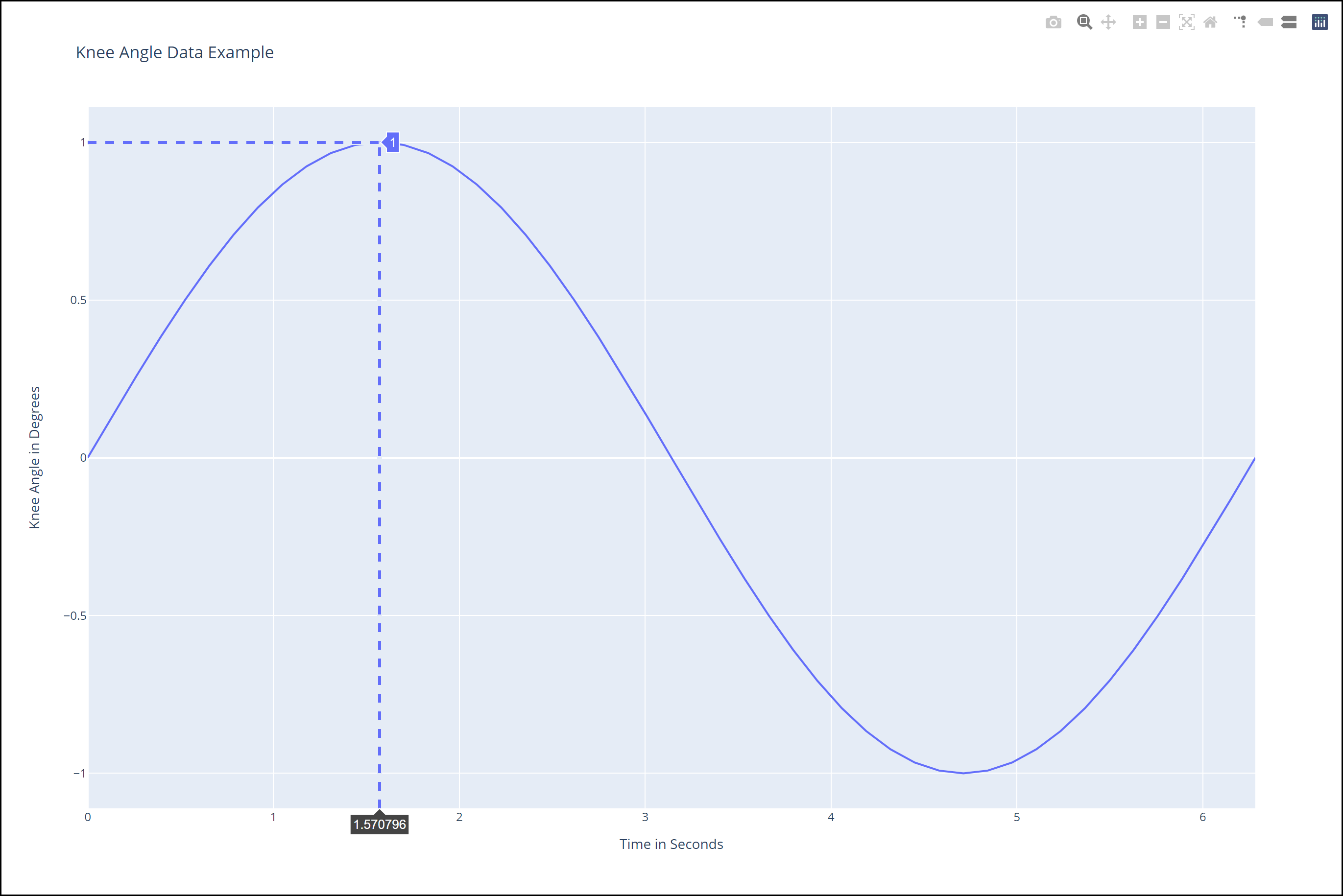

This marks the end of the program.

Appendix

Optional refactor 0:

• Use try-except-*else* and/or try-except-*finally* blocks.

Optional refactor 1:

xxxxxxxxxx
1  try:
2  │   ser = Serial(port)
3  except:
4  │   ...

to

xxxxxxxxxx
1  from serial.tools.list_ports import comports
2  
3  if port in [comport.device for comport in comports()]:
4  │   ser = Serial(port)
5  elif:
6  │   ...

However, between lines 3 and 4 above, the serial port might become unavailable, in which case Serial would throw an uncaught SerialException error.

Optional refactor 2:

xxxxxxxxxx
1  try:
2  │   ser.readline()
3  except:
4  │   ...

to

xxxxxxxxxx
1  from serial.tools.list_ports import comports
2  
3  if port not in [comport.device for comport in comports()]:
4  │   ...

 

---

 

Example: A More Complex Application in a Simple Windows UI…

The following fully-assembled Python module/script runs a very simple Windows UI for interfacing with an RC car, all made by me.

from serial import Serial
from win10toast import ToastNotifier
from time import time
from threading import Thread
import ctypes
import tkinter as tk
toaster = ToastNotifier()
port = 'COM4'  # 'COM3'
try:
    ser = Serial(port, baudrate = 115_200)
except:
    while True:
        if toaster.show_toast('Connect the BLE link via USB', ' ',
                              icon_path = 'ico/connect.ico',
                              threaded = True):
            break
        try:
            ser = Serial(port, baudrate = 115_200)
            break
        except:
            pass
    try:
        ser
    except:
        while True:
            try:
                ser = Serial(port, baudrate = 115_200)
                break
            except:
                pass
connected_notified = False
def connected_notifier():
    global connected_notified
    connected_tick = time()
    while True:
        connected_tock = time()
        connected_time = connected_tock - connected_tick
        if toaster.show_toast('BLE link connected',
                              '%.1f seconds ago' % connected_time,
                              icon_path = 'ico/connected.ico',
                              threaded = True):
            connected_notified = True
            break
        print('connected_notifier waiting')
Thread(target = connected_notifier).start()
ctypes.windll.shcore.SetProcessDpiAwareness(True)
window = tk.Tk()
# window.resizable(False, False)
window.configure(bg = 'white')
window.iconbitmap('ico/window.ico')
window.title('RC Car Interface')
with open('rc_car_interface_instructions.txt') as file:
    instructions = ''.join(file.readlines())
label = tk.Label(text = instructions, justify = tk.LEFT, font = ('Segoe UI Semilight', 12))
label.config(bg = 'white')
label.pack(padx = 100, pady = 100)
def disconnected_notifier():
    disconnected_tick = time()
    while True:
        disconnected_tock = time()
        if connected_notified:
            disconnected_time = disconnected_tock - disconnected_tick
            if toaster.show_toast('BLE link disconnected',
                                  '%.1f seconds ago' % disconnected_time,
                                  icon_path = 'ico/disconnected.ico',
                                  threaded = True):
                break
        print('disconnected_notifier waiting')
disconnected = False
closed = False
def disconnected_checker():
    global disconnected
    while True:
        if not closed:
            try:
                ser.read()
            except:
                disconnected = True
                try:
                    window.destroy()
                    window.quit()
                except:
                    pass
                disconnected_notifier()
                break
        else:
            break
        print('disconnected_checker waiting')
Thread(target = disconnected_checker).start()
commands = ['v', 'l', 'B', 'r', 'a', 's', 'b', 'L', 'F', 'R']
with open('rc_car_interface_actions.txt') as file:
    actions = file.readlines()
def keypress_handler(event):
    try:
        index = int(event.char)
        command = commands[index]
        action = actions[index]
        ser.write(command.encode())
        print(action[:-1])
    except:
        try:
            ser.write(b's')
            window.destroy()
            window.quit()
        except:
            pass
    print('keypress_handler called')
window.bind('<Key>', keypress_handler)
window.mainloop()
closed = True
if not disconnected:
    def closed_notifier():
        closed_tick = time()
        while True:
            closed_tock = time()
            if connected_notified:
                closed_time = closed_tock - closed_tick
                if toaster.show_toast('BLE link interface closed',
                                      '%.1f seconds ago' % closed_time,
                                      icon_path = 'ico/closed.ico',
                                      threaded = True):
                    break
            print('closed_notifier waiting')
    Thread(target = closed_notifier).start()
ser.__del__()

---

---